Gazebo robotics simulator with ROS
This tutorial is intended for roboticists that want to have realistic simulations of their robotic scenarios. Gazebo is a 3D simulator, while ROS serves as the interface for the robot. Combining both results in a powerful robot simulator.
With Gazebo you are able to create a 3D scenario on your computer with robots, obstacles and many other objects. Gazebo also uses a physical engine for illumination, gravity, inertia, etc. You can evaluate and test your robot in difficult or dangerous scenarios without any harm to your robot. Most of the time it is faster to run a simulator instead of starting the whole scenario on your real robot.
Originally Gazebo was designed to evaluate algorithms for robots. For many applications it is essential to test your robot application, like error handling, battery life, localization, navigation and grasping. As there was a need for a multi-robot simulator Gazebo was developed and improved.
This Tutorial was tested with an Ubuntu 12.10 with ROS Hydro and Gazebo-1.9.
Sources
Sources for this tutorial can be found on GitHub
Installation of Gazebo
For Gazebo there are also multiple options for installation. As I use an Ubuntu I selected the installation with precompiled binaries. Make sure you can launch “gzserver” and “gzclient” after the installation of Gazebo.
Gazebo is split up in two parts. The server part computes all the physics and world, while the client is the graphical frontent for gazebo. So if you want to save performance on your computer you could also execute all tests without the graphical interface. Although it looks very nice, it consumes a lot of resources.
Your Gazebo should be installed in:
/usr/bin/gzserver/usb/bin/gzclient
or
/usr/local/bin/gzserver/usr/local/bin/gzclient
if you installed Gazebo from sources.
After Gazebo and ROS have been installed it is time to install the bridge between them. With this bridge you can launch gazebo within ROS and dynamically add models to Gazebo. Depending on your Gazebo installation, there are different methods to continue.
If you have ROS Hydro you probably want to follow this guide to install the ROS Packages for Gazebo and look at the ‘Install Pre-Built Debians’ section.
If you do not have the ROS Version “Hydro” installed, you have to manually “git clone” the “gazebo_ros_pkgs”. The git url can be found on http://www.ros.org/wiki/gazebo_ros_pkgs. If git is not installed:
sudo apt-get install git
If you have some missing dependencies, the following two packages may help
sudo apt-get install ros-hydro-pcl-conversionssudo apt-get install ros-hydro-control-msgs
If the cmake_modules are missing, “git clone” them in the sources of your catkin directory.
git clone https://github.com/ros/cmake_modules
If everything worked you should be able to start Gazebo and ROS with (remember to source your environment):
roscore & rosrun gazebo_ros gazebo
You could also start them individually with gzserver and gzclient. If Gazebo is properly connected to ROS you should be able to the some published topics. Just type
rostopic list
in one of your favorite terminals to see, if there are some gazebo topics if the gzserver is running.
/gazebo/link_states/gazebo/model_states/gazebo/parameter_descriptions/gazebo/parameter_updates/gazebo/set_link_state/gazebo/set_model_state
First Steps with Gazebo and ROS
You should have previously installed Gazebo and ROS. Now you are ready to discover the fascinating world of simulation. In this tutorial we are going to:
•setup a ROS workspace
•create projects for your simulated robot
•create a Gazebo world
•create your own robot model
•connect your robot model to ROS
•use a teleoperation node to control your robot
•add a camera to your robot
•use Rviz to vizualize all the robot information
Setup a new workspace
We’ll assume that you start from scratch and need to create a new workspace for your project. Let’s first source our ROS Hydro environment:
source /opt/ros/hydro/setup.bashNow let’s create the folder that will contain our workspace and the ‘src’ subfolder.
mkdir -p ~/catkin_ws/srcGo into the source and initialize the workspace:
cd ~/catkin_ws/srccatkin_init_workspaceLets do a first build of your (empty) workspace just to generate the proper setup files
cd ..catkin_makeFrom now on, each time we’ll have to start ROS commands that imply using our packages, we’ll have to source the workspace environment in each terminal:
source ~/catkin_ws/devel/setup.bashCreate projects for your simulated robot
The ROS community has established some conventions for packages that define robots, their ROS bindings and the Gazebo integration. We’ll try to follow these conventions for this simple robot. Let’s assume our robot will be called mybot. We are going to create 3 packages:
mybot_gazebo: provides launch files and worlds for easy starting of simulation mybot_description: provides the 3D model of the robot and the description of joints and sensors mybot_control: configures the ROS interface to our robot’s joints Ok let’s create these, first make sure you’ve sourced your workspace environment and go into the ‘src’ subfolder:
cd ~/catkin_ws/srcLet’s create the three packages:
catkin_create_pkg mybot_gazebo gazebo_roscatkin_create_pkg mybot_descriptioncatkin_create_pkg mybot_controlCreating your own World
Let’s start with the gazebo package, go in there and create the following subfolders:
roscd mybot_gazebo mkdir launch worldsAt first we want to create a world for our gazebo server. Therefore we switch to our worlds directory of our turtlebot project and create a new world file.
cd worldsgedit mybot.worldA basic world file defines at least a name:
<?xml version="1.0"?>
<sdf version="1.4">
<world name="myworld">
</world>
</sdf>
Here you could directly add models and object with their position. Also the laws of physics may be defined in a world. This is an important step to understand, because in this file you could also attach a specific plugin to an object. The plugin itself contains ROS and Gazebo specific code for more complex behaviors.
At first we just want to add some basic objects, like a ground and a basic illumination source inside the world tag.
	<include>
		<uri>model://sun</uri>
	</include>

	<include>
		<uri>model://ground_plane</uri>
	</include>
Check your “~/.gazebo/models” directory, as this is a default path for saved models. If this path does not exist try to find /usr/share/gazebo/setup.sh where gazebo looks for models. Otherwise add it to your model path.
As the ground plane and the sun are basic models that are also on the gazebo server they will be downloaded on startup if they cannot be found locally. If you want to know which object are available on the gazebo server, take a look at Gazebo model database. To start the gazebo server there are several methods. As it is a good practice to use a launch file, we will create one now. This could later also be used for multiple nodes.
Change to the launch directory of your project:
roscd mybot_gazebo/launchCreate a new file:
gedit mybot_world.launchand insert:
<launch>
	<include file="$(find gazebo_ros)/launch/empty_world.launch">
		<arg name="world_name" value="$(find mybot_gazebo)/worlds/mybot.world"/>
		<arg name="gui" value="true"/>
	</include>
</launch>
This launch file will just execute a default launch file provided by Gazebo, and tell it to load our world file and show the Gazebo client. You can launch it by doing:
roslaunch mybot_gazebo mybot_world.launchNow you should see the gazebo server and the gui starting with a world that contains a ground plane and a sun (which is not obviously visible without objects). If not, it can be that there are some connections problems with the server.
If that happens, start gazebo without the launch file, go to the models, you should find the one you want in the server. Click on them, they will be put in the cache. Now, if you close gazebo and start it again with the launch file, it should work.
If you would press “Save world as” in “File” in your gazebo client and save the world in a text file, you could investigate the full world description.
If you want to watch a more complex and beautiful world environment then add the following inside your world tag:
  	<include>
		<uri>model://willowgarage</uri>
	</include>
This one shows you the office of Willow Garage, be careful, it’s huge and may make your simulation extremely slow.
Creating your own Model
The more accurate you want to model your robot the more time you need to spend on the design. In the next image you see a developing process of a robot model, from a simple cube to a differential drive robot. You can also check the ROS tutorial about the robot.
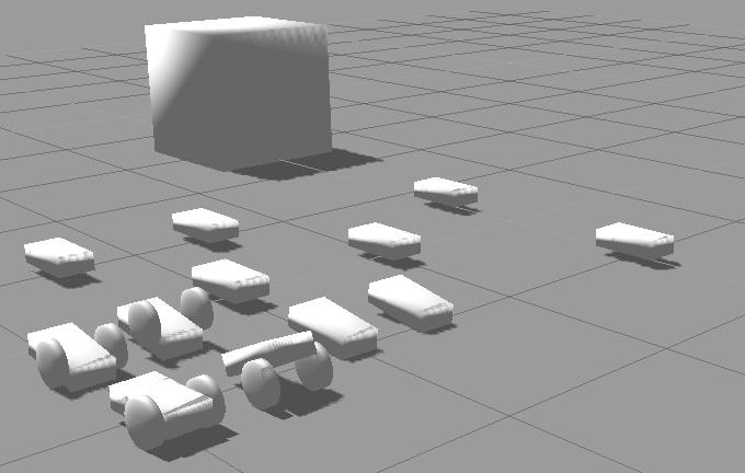
We could put our model as a SDF file in the ~/.gazebo/models directory, this is the standard way when you work only with Gazebo. However with ROS we’ll prefer to use a URDF file generated by Xacro and put it the description package.
The Universal Robotic Description Format (URDF) is an XML file format used in ROS as the native format to describe all elements of a robot. Xacro (XML Macros) is an XML macro language. It is very useful to make shorter and clearer robot descriptions.
Ok so first we need to go into our description package and create the urdf subfolder and the description file:
roscd mybot_descriptionmkdir urdfcd urdfgedit mybot.xacroXACRO CONCEPTS
• xacro:include: Import the content from other file. We can divide the content in different xacros and merge them using xacro:include.
• property: Useful to define constant values. Use it later using ${property_name}
• xacro:macro: Macro with variable values. Later, we can use this macro from another xacro file, and we specify the required value for the variables. To use a macro, you have to include the file where the macro is, and call it using the macro’s name and filling the required values.
This file will be the main description of our robot. Let’s put some basic structure:
<?xml version="1.0"?>
<robot name="mybot" xmlns:xacro="http://www.ros.org/wiki/xacro">
        <!-- Put here the robot description -->
</robot>
The structure is basic for a urdf file. The complete description (links, joints, transmission…) have to be within the robot tag. The xmlns:xacro="http://www.ros.org/wiki/xacro" specifies that this file will use xacro. If you want to use xacro you have to put this.
With xacro, you can define parameters. Once again, this make the file clearer. They are usually put at the beginning of the file (within the robot tag, of course).
Let’s define some physical properties for our robot, mainly the dimensions of the chassis, the caster wheel, the wheels and the camera:
<xacro:property name="PI" value="3.1415926535897931"/>

<xacro:property name="chassisHeight" value="0.1"/>
<xacro:property name="chassisLength" value="0.4"/>
<xacro:property name="chassisWidth" value="0.2"/>
<xacro:property name="chassisMass" value="50"/>

<xacro:property name="casterRadius" value="0.05"/>
<xacro:property name="casterMass" value="5"/>

<xacro:property name="wheelWidth" value="0.05"/>
<xacro:property name="wheelRadius" value="0.1"/>
<xacro:property name="wheelPos" value="0.2"/>
<xacro:property name="wheelMass" value="5"/>

<xacro:property name="cameraSize" value="0.05"/>
<xacro:property name="cameraMass" value="0.1"/>
‹arg name="gui" value="true"/›These parameters or properties can be used in all the file with ${property name}.
We will also include three files :
 <xacro:include filename="$(find mybot_description)/urdf/mybot.gazebo" />
 <xacro:include filename="$(find mybot_description)/urdf/materials.xacro" />
 <xacro:include filename="$(find mybot_description)/urdf/macros.xacro" />
These three correspond respectively to:
• all the gazebo-specific aspects of our robot
• definition of the materials used (mostly colors)
• definitions of some macros for easier description of the robot
Every file has to contain the robot tag and everything we put in them should be in this tag.
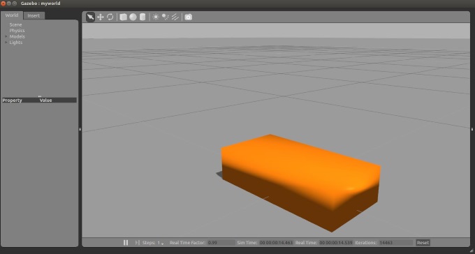
Now we want to add a rectangular base for our robot. Insert this within the robot tag of mybox.xacro:
<link name='chassis'>
  <collision>
    <origin xyz="0 0 ${wheelRadius}" rpy="0 0 0"/>
    <geometry>
      <box size="${chassisLength} ${chassisWidth} ${chassisHeight}"/>
    </geometry>
  </collision>
  <visual>
    <origin xyz="0 0 ${wheelRadius}" rpy="0 0 0"/>
    <geometry>
      <box size="${chassisLength} ${chassisWidth} ${chassisHeight}"/>
    </geometry>
    <material name="orange"/>
  </visual>
  <inertial>
    <origin xyz="0 0 ${wheelRadius}" rpy="0 0 0"/>
    <mass value="${chassisMass}"/>
    <box_inertia m="${chassisMass}" x="${chassisLength}" y="${chassisWidth}" z="${chassisHeight}"/>
  </inertial>
</link>
We define a box with chassisLength x chassisWidth x chassisHeight meters and mass chassisMasskg.
As you can see, we have three tags for this one box, where one is used to the collision detection engine, one to the visual rendering engine and the last to the physic engine. Most of the time they are the same, except when you have complicated and beautiful visual meshes.
As they don’t need to be that complicated for collision detection you could use a simple model for the collision. The material element in the visual tag refer to a color that must be defined in the materials.xacro and refred to in the mybot.gazebo file, at least, in the structure we adopted.
Add this in “mybot.gazebo”, within the robot tag :
<gazebo reference="chassis">
  <material>Gazebo/Orange</material>
</gazebo>
And this in the “materials.xacro” :
<material name="black">
  <color rgba="0.0 0.0 0.0 1.0"/>
</material>

<material name="blue">
  <color rgba="0.0 0.0 0.8 1.0"/>
</material>

<material name="green">
  <color rgba="0.0 0.8 0.0 1.0"/>
</material>

<material name="grey">
  <color rgba="0.2 0.2 0.2 1.0"/>
</material>

<material name="orange">
  <color rgba="${255/255} ${108/255} ${10/255} 1.0"/>
</material>

<material name="brown">
  <color rgba="${222/255} ${207/255} ${195/255} 1.0"/>
</material>

<material name="red">
  <color rgba="0.8 0.0 0.0 1.0"/>
</material>

<material name="white">
  <color rgba="1.0 1.0 1.0 1.0"/>
</material>
As you can see, we add more than just the color we wanted, this is for convenience. Now, we can leave this file alone and use any color we want.
Another particular thing in the chassis link is the use of “box_inertia” in the inertial tag. This is a macro made with xacro. As you can see, when you use a macro, you can simply use the tag and specifies the parameters. Xacro will understand.
Add this in the macros.xacro file, within the robot tag :
<macro name="cylinder_inertia" params="m r h">
  <inertia  ixx="${m*(3*r*r+h*h)/12}" ixy = "0" ixz = "0"
    iyy="${m*(3*r*r+h*h)/12}" iyz = "0"
    izz="${m*r*r/2}"
  />
</macro>

<macro name="box_inertia" params="m x y z">
  <inertia  ixx="${m*(y*y+z*z)/12}" ixy = "0" ixz = "0"
    iyy="${m*(x*x+z*z)/12}" iyz = "0"
    izz="${m*(x*x+z*z)/12}"
  />
</macro>

<macro name="sphere_inertia" params="m r">
  <inertia  ixx="${2*m*r*r/5}" ixy = "0" ixz = "0"
    iyy="${2*m*r*r/5}" iyz = "0"
    izz="${2*m*r*r/5}"
  />
</macro>
Once again, we add more than we needed. We will use the others later. The inertia tag is a convention of the inertial tag in a link.
We have two small things to do before testing our model with gazebo.
The physic engine does not accept a base_link with inertia. It is then useful to add a simple link without inertia and make a joint between it and the chassis. Add this before the chassis link in the mybot.xacro file :
<link name="footprint" />

<joint name="base_joint" type="fixed">
  <parent link="footprint"/>
  <child link="chassis"/>
</joint>
In order to start gazebo with our model, we have to modify the previously created launch file mybot_world.launch by adding the following two tags in the launch tag:
<!-- urdf xml robot description loaded on the Parameter Server, converting the xacro into a proper urdf file-->
<param name="robot_description" command="$(find xacro)/xacro.py '$(find mybot_description)/urdf/mybot.xacro'" />

<!-- push robot_description to factory and spawn robot in gazebo -->
<node name="mybot_spawn" pkg="gazebo_ros" type="spawn_model" output="screen"
 args="-urdf -param robot_description -model mybot" />
The first tag will first call the xacro script to convert of xacro description into an actual URDF. This URDF is then inserted into a ROS parameter called “robot_description” (this is a standard name used by many ROS tools).
The second tag launches a program from the gazebo_ros package that will load the URDF from the parameter “robot_description” and spawn the model into our Gazebo simulator
If you launch your project with this launch file, the gazebo client opens and the the chassis should be there. It should also fall because of the physic engine.
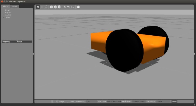
As a next step we add a caster wheel to the robot. This is the simplest wheel as we have no axis and no friction. We can simply approximate the caster wheel with a ball. Add this after the chassis link in the main urdf file :
<joint name="fixed" type="fixed">
  <parent link="chassis"/>
  <child link="caster_wheel"/>
</joint>

<link name="caster_wheel">
  <collision>
    <origin xyz="${casterRadius-chassisLength/2} 0 ${casterRadius-chassisHeight+wheelRadius}" rpy="0 0 0"/>
    <geometry>
      <sphere radius="${casterRadius}"/>
    </geometry>
  </collision>

  <visual>
    <origin xyz="${casterRadius-chassisLength/2} 0 ${casterRadius-chassisHeight+wheelRadius}" rpy="0 0 0"/>
    <geometry>
      <sphere radius="${casterRadius}"/>
    </geometry>
    <material name="red"/>
  </visual>

  <inertial>
    <origin xyz="${casterRadius-chassisLength/2} 0 ${casterRadius-chassisHeight+wheelRadius}" rpy="0 0 0"/>
    <mass value="${casterMass}"/>
    <sphere_inertia m="${casterMass}" r="${casterRadius}"/>
  </inertial>
</link>
We attach this caster wheel to the chassis with a fixed joint. The two links will then always move together. We use the sphere_inertia macro we added earlier in the macros.xacro file. Also add a gazebo tag in the gazebo file for this link :
<gazebo reference="caster_wheel">
  <mu1>0.0</mu1>
  <mu2>0.0</mu2>
  <material>Gazebo/Red</material>
</gazebo>
As usual, we specify the color used in material. We also added mu1 and mu2, with value 0 to remove the friction.
Last but not least, we want to add some wheels to the robot. We could add the two links in the main file, but let’s make one macro to make it simple. In the macro file, add this :
<macro name="wheel" params="lr tY">

<link name="${lr}_wheel">
  <collision>
    <origin xyz="0 0 0" rpy="0 ${PI/2} ${PI/2}" />
    <geometry>
      <cylinder length="${wheelWidth}" radius="${wheelRadius}"/>
    </geometry>
  </collision>

  <visual>
    <origin xyz="0 0 0" rpy="0 ${PI/2} ${PI/2}" />
    <geometry>
      <cylinder length="${wheelWidth}" radius="${wheelRadius}"/>
    </geometry>
    <material name="black"/>
  </visual>

  <inertial>
    <origin xyz="0 0 0" rpy="0 ${PI/2} ${PI/2}" />
    <mass value="${wheelMass}"/>
    <cylinder_inertia m="${wheelMass}" r="${wheelRadius}" h="${wheelWidth}"/>
  </inertial>
</link>

<gazebo reference="${lr}_wheel">
  <mu1 value="1.0"/>
  <mu2 value="1.0"/>
  <kp  value="10000000.0" />
  <kd  value="1.0" />
  <fdir1 value="1 0 0"/>
  <material>Gazebo/Black</material>
</gazebo>


<joint name="${lr}_wheel_hinge" type="continuous">
  <parent link="chassis"/>
  <child link="${lr}_wheel"/>
<origin xyz="${-wheelPos+chassisLength/2} ${tY*wheelWidth/2+tY*chassisWidth/2} ${wheelRadius}" rpy="0 0 0" />
  <axis xyz="0 1 0" rpy="0 0 0" />
  <limit effort="100" velocity="100"/>
  <joint_properties damping="0.0" friction="0.0"/>
</joint>


<transmission name="${lr}_trans">
  <type>transmission_interface/SimpleTransmission</type>
  <joint name="${lr}_wheel_hinge"/>
  <actuator name="${lr}Motor">
    <hardwareInterface>EffortJointInterface</hardwareInterface>
    <mechanicalReduction>10</mechanicalReduction>
  </actuator>
</transmission>

</macro>
The parameters allows us to specify which wheel we are talking about. “lr” could have two values (left or right) and “tY”, for translation along the Y-axis, also (respectively 1 and -1). There is nothing new concerning the link part.
The gazebo tag is inserted here so that we don’t need to worry about it every time we add a wheel. This macro is thus self-sufficient. The joint type is continuous. This allows a rotation around one axis. This axis is y 0 1 0 and connects each wheel to the chassis of your robot.
What’s new is the transmission element. To use ros_control with your robot, you need to add some additional elements to your URDF. The element is used to link actuators to joints, see the spec for exact XML format. We’ll use them in a minute.
Now you can add the wheels to the main file :
<wheel lr="left" tY="1"/>
<wheel lr="right" tY="-1"/>
As you see, the macro makes it very simple.
Now you can launch your simulation and the full robot should appear!
Connect your robot to ROS
Alright, our robot is all nice and has this new car smell, but we can’t do anything with it yet as it has no connection with ROS. In order to add this connection we need to add gazebeo plugins to our model. There are different kinds of plugins:
• World: Dynamic changes to the world, e.g. Physics, like illumination or gravity, inserting models
• Model: Manipulation of models (robots), e.g. move the robots
• Sensor: Feedback from virtual sensor, like camera, laser scanner
• System: Plugins that are loaded by the GUI, like saving images
First of all we’ll use a plugin to provide access to the joints of the wheels. The transmission tags in our URDF will be used by this plugin the define how to link the joints to controllers. To activate the plugin, add the following to mybot.gazebo:
<gazebo>
  <plugin name="gazebo_ros_control" filename="libgazebo_ros_control.so">
    <robotNamespace>/mybot</robotNamespace>
  </plugin>
</gazebo>
Look at this tutorial for more information on how this plugin works.
With this plugin, we will be able to control the joints, however we need to provide some extra configuration and explicitely start controllers for the joints. In order to do so, we’ll use the package mybot_control that we have defined before. Let’s first create the configuration file:
roscd mybot_controlmkdir configcd configgedit mybot_control.yamlThis file will define three controllers: one for each wheel, connections to the joint by the transmission tag, one for publishing the joint states. It also defined the PID gains to use for this controller:
mybot:
  # Publish all joint states -----------------------------------
  joint_state_controller:
    type: joint_state_controller/JointStateController
    publish_rate: 50


  # Effort Controllers ---------------------------------------
  leftWheel_effort_controller:
    type: effort_controllers/JointEffortController
    joint: left_wheel_hinge
    pid: {p: 100.0, i: 0.1, d: 10.0}
  rightWheel_effort_controller:
    type: effort_controllers/JointEffortController
    joint: right_wheel_hinge
    pid: {p: 100.0, i: 0.1, d: 10.0}
Now we need to create a launch file to start the controllers. For this let’s do:
roscd mybot_controlmkdir launchcd launchgedit mybot_control.launchIn this file we’ll put two things. First we’ll load the configuration and the controllers, and we’ll also start a node that will provide 3D transforms (tf) of our robot. This is not mandatory but that makes the simulation more complete:
<launch>

  <!-- Load joint controller configurations from YAML file to parameter server -->
  <rosparam file="$(find mybot_control)/config/mybot_control.yaml" command="load"/>

  <!-- load the controllers -->
  <node name="controller_spawner"
    pkg="controller_manager"
    type="spawner" respawn="false"
    output="screen" ns="/mybot"
    args="joint_state_controller
      rightWheel_effort_controller
      leftWheel_effort_controller"
  />


  <!-- convert joint states to TF transforms for rviz, etc -->
  <node name="robot_state_publisher" pkg="robot_state_publisher" type="robot_state_publisher" respawn="false" output="screen">
    <param name="robot_description" command="$(find xacro)/xacro.py '$(find mybot_description)/urdf/mybot.xacro'" />
    <remap from="/joint_states" to="/mybot/joint_states" />
  </node>

</launch>
We could launch our model on gazebo and then launch the controller, but to save some time (and terminals), we’ll start the controllers automatically by adding a line to the “mybot_world.launch” in the mybot_gazebo package :
<!-- ros_control mybot launch file -->
<include file="$(find mybot_control)/launch/mybot_control.launch" />
Now launch your simulations. In a separate terminal, if you do a “rostopic list” you should see the topics corresponding to your controllers. You can send commands manually to your robot:
  rostopic pub -1 /mybot/leftWheel_effort_controller/command std_msgs/Float64 "data: 1.5"
  rostopic pub -1 /mybot/rightWheel_effort_controller/command std_msgs/Float64 "data: 1.0"
The robot should start moving. Congratulations, you can now control your joints through ROS ! You can also monitor the joint states by doing :
rostopic echo /mybot/joint_statesTeleoperation of your robot
Ok you can control joints individually, but that’s not so convenient when you want to make your mobile robot move around. Let’s use another plugin called differential drive to make it easier. Add this in the gazebo file of your model :
<gazebo>
  <plugin name="differential_drive_controller" filename="libgazebo_ros_diff_drive.so">
    <alwaysOn>true</alwaysOn>
    <updateRate>100</updateRate>
    <leftJoint>left_wheel_hinge</leftJoint>
    <rightJoint>right_wheel_hinge</rightJoint>
    <wheelSeparation>${chassisWidth+wheelWidth}</wheelSeparation>
    <wheelDiameter>${2*wheelRadius}</wheelDiameter>
    <torque>20</torque>
    <commandTopic>mybot/cmd_vel</commandTopic>
    <odometryTopic>mybot/odom_diffdrive</odometryTopic>
    <odometryFrame>odom</odometryFrame>
    <robotBaseFrame>footprint</robotBaseFrame>
  </plugin>
</gazebo>
This plugin will subscribe to the cmd_vel topic specified with the « commandTopic » tag and convert the messages to the proper commands on the wheels. It also provides some odometry data.
Now, you can start gazebo with the usual launch file.
To teleoperate your robot with the keybord you can use a teleoperation node as provided in turtlesim or turtlebot packages. We just need to remap the topic name to connect it to our robot :
	rosrun turtlesim turtle_teleop_key /turtle1/cmd_vel:=/mybot/cmd_vel
	rosrun turtlebot_teleop turtlebot_teleop_key /turtlebot_teleop/cmd_vel:=/mybot/cmd_vel
Enjoy the ride !
Adding a camera
Let’s add some sensors to our robot. If you already created some environment, you can now see what it is, with the eyes of your robot. For this we have to add a camera plugin to our robot model. For that, two things are necessary, a link and the actual plugin.
Add the link to your main model file :
<link name="camera">
  <collision>
    <origin xyz="0 0 0" rpy="0 0 0"/>
    <geometry>
      <box size="${cameraSize} ${cameraSize} ${cameraSize}"/>
    </geometry>
  </collision>

  <visual>
    <origin xyz="0 0 0" rpy="0 0 0"/>
    <geometry>
      <box size="${cameraSize} ${cameraSize} ${cameraSize}"/>
    </geometry>
    <material name="blue"/>
  </visual>

  <inertial>
    <mass value="${cameraMass}" />
    <origin xyz="0 0 0" rpy="0 0 0"/>
    <box_inertia m="${cameraMass}" x="${cameraSize}" y="${cameraSize}" z="${cameraSize}" />
  </inertial>
</link>
And now add the plugin to the gazebo file:
<gazebo reference="camera">
  <material>Gazebo/Blue</material>
  <sensor type="camera" name="camera1">
    <update_rate>30.0</update_rate>
    <camera name="head">
      <horizontal_fov>1.3962634</horizontal_fov>
      <image>
        <width>800</width>
        <height>800</height>
        <format>R8G8B8</format>
      </image>
      <clip>
        <near>0.02</near>
        <far>300</far>
      </clip>
    </camera>
    <plugin name="camera_controller" filename="libgazebo_ros_camera.so">
      <alwaysOn>true</alwaysOn>
      <updateRate>0.0</updateRate>
      <cameraName>mybot/camera1</cameraName>
      <imageTopicName>image_raw</imageTopicName>
      <cameraInfoTopicName>camera_info</cameraInfoTopicName>
      <frameName>camera_link</frameName>
      <hackBaseline>0.07</hackBaseline>
      <distortionK1>0.0</distortionK1>
      <distortionK2>0.0</distortionK2>
      <distortionK3>0.0</distortionK3>
      <distortionT1>0.0</distortionT1>
      <distortionT2>0.0</distortionT2>
    </plugin>
  </sensor>
 </gazebo>Adding a camera

Let's add some sensors to our robot. If you already created some environment, you can now see what it is, with the eyes of your robot.
Launch your simulation, and add some object in front of the robot. You can obtain the camera image as with any ROS compatible camera, by subscribing to the image topic. You can use the image_view tool to visualize it directly:
rosrun image_view image_view image:=/mybot/camera1/image_raw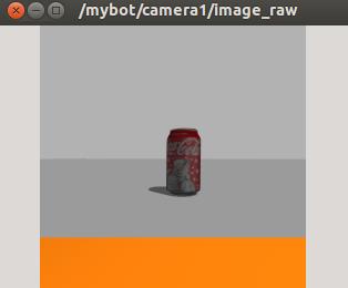
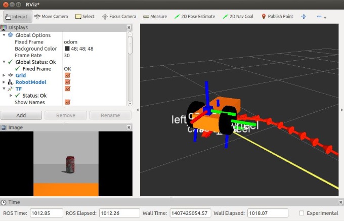
Visualisation with RViz
Rviz is one of these fantastic tools that will make you love ROS. It’s capable of visualizing many different kind of information in the same interface. To start rviz:
rosrun rviz rvizAt the bottom left of the window there is an “add” button which allows you to load visualization plugins. In the parameters of these plugins you generally have to define the topic name to which the plugin subscribes, this should be fairly straightforward. A Rviz configuration file is provided with the sources and started by default in the launch file.
Here is an example visualization with plugins for: the robot model, the 3D transforms TF, the camera Image, the odometry: